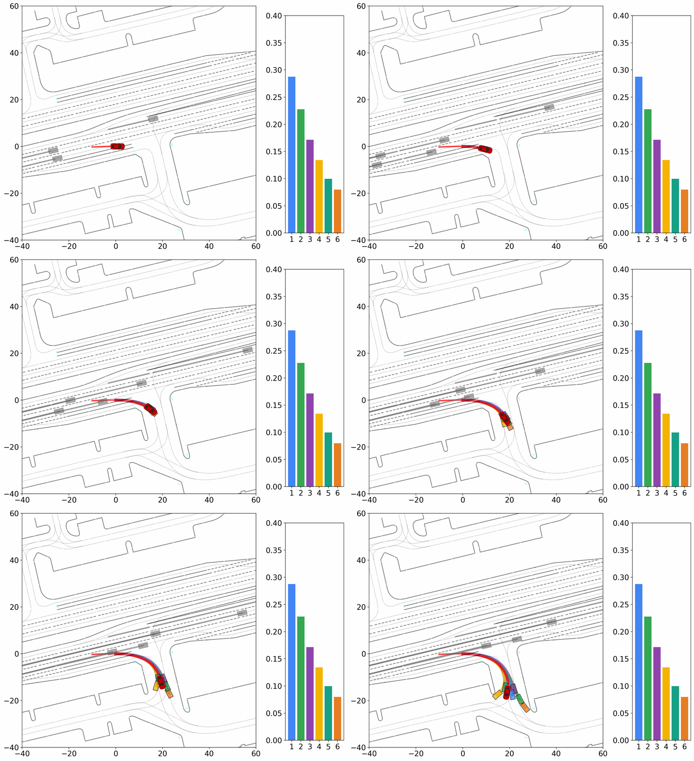
Conditional Generative Models for Motion Prediction
In this blog post, we discuss good engineering practices and the lessons learned—sometimes the hard way—from building conditional generative models (in particular, flow matching) for motion prediction problems.
Introduction
Needless to say, diffusion-based generative models (equivalently, flow matching models) are amazing inventions. They have shown great capacity to produce high-quality images, videos, audios and more, whether being unconditional on the benchmark datasets and conditioned on certain content in the wild. In this blog, we discuss a relatively less explored application of generative models for motion prediction, which is a fundamental problem in many applications such as autonomous driving and robotics.
In a nutshell, motion prediction is the task of predicting the future trajectories of objects given their past trajectories, plus all sorts of available context information such as surrounding objects and high-fidelity maps.
The said pipeline implemented by neural networks is simply:
Past Trajectory + Context Information ---> Neural Network ---> Future Trajectory
To produce meaningful future trajectories, we condition the generative models on the past trajectory and the context information. Borrowed from our paper

The early datasets on human motion prediction mostly do not come with heavy context information, such as the well-known ETH-UCY and the SDD datasets (see more for summarization at
Challenges of Multi-Modal Prediction
Motion prediction, as the name suggests, is inherently a forecasting task. For each input in a dataset, only one realization of the future motion is recorded, even though multiple plausible outcomes often exist. This mismatch between the inherently multi-modal nature of future motion and the single ground-truth annotation poses a core challenge for evaluation.
In practice, standard metrics require models to output multiple trajectories, which are then compared against the observed ground truth. For example, ADE (Average Displacement Error) and FDE (Final Displacement Error) measure trajectory errors, and the minimum ADE/FDE across predictions is typically reported. This setup implicitly encourages models to produce diverse hypotheses, but only rewards the one closest to the recorded future. Datasets such as Waymo Open Motion

The strong dependency of current evaluation metrics on a single ground truth, assessed instance by instance, poses a particular challenge for generative models. Although the task inherently requires generating diverse trajectories, models are only rewarded when one of their outputs happens to align closely with the recorded ground truth.
As a result, the powerful ability of generative models to produce diverse samples from noise
Engineering Practices and Lessons
Now let’s dive into the technical side of the problem. In the forward process of flow matching, we adopt a simple linear interpolation between the clean trajectories \(Y^1 \sim q\), where \(q\) is the data distribution, and pure Gaussian noise \(Y^0 \sim \mathcal{N}(\mathbf{0}, \mathbf{I})\):
\[Y^t = (1-t)Y^0 + tY^1 \qquad t \in [0, 1].\]The reverse process, which allows us to generate new samples, is governed by the ordinary differential equations (ODEs):
\[\mathrm{d} Y^t = v_\theta(Y^t, t, C)\mathrm{d}t,\]where \(v_\theta\) is the parametrized vector field approximating the straight flow \(U^t = Y^1 - Y^0\). Here, \(C\) denotes the aggregated contextual information of agents in a scene, including the past trajectory and any other available context information.
Data-Space Predictive Learning Objectives
From an engineering standpoint, a somewhat bitter lesson we encountered is that existing predictive learning objectives remain remarkably strong. Despite the appeal of noise-prediction formulations (e.g., $\epsilon$-prediction introduced in DDPM
Concretely, by rearranging the original linear flow objective, we define a neural network
\[D_\theta := Y^t + (1-t)v_\theta(Y^t, C, t),\]which is trained to recover the future trajectory \(Y^1\) in the data space. The corresponding objective is:
\[\mathcal{L}_{\text{FM}} = \mathbb{E}_{Y^t, Y^1 \sim q, \, t \sim \mathcal{U}[0,1]} \left[ \frac{\| D_{\theta}(Y^t, C, t) - Y^1 \|_2^2}{(1 - t)^2} \right].\]Our empirical observation is that data-space predictive learning objectives outperform denoising objectives. We argue that this is largely influenced by the current evaluation protocol, which heavily rewards model outputs that are close to the ground truth.
During training, the original denoising target matches the vector field $Y^1 - Y^0$, defined as the difference between the data sample (future trajectory) and the noise sample (drawn from the noise distribution). Under the current proximity-based metrics, this objective is harder to optimize than the predictive objective because of the stochasticity introduced by $Y^0$, as the metrics do not adequately reward diverse forecasting. Moreover, during the sampling process, small errors in the vector field model $v_\theta$—measured with respect to the single ground-truth velocity field at intermediate time steps—can be amplified through subsequent iterative steps. Consequently, increasing inference-time compute may not necessarily improve results without incorporating regularization from the data-space loss
Joint Multi-Modal Learning Losses
Building on this, another key engineering practice was to introduce joint multi-modal learning losses. Our network \(D_\theta\) generates \(K\) scene-level correlated waypoint predictions \(\{S_i\}_{i=1}^K\) along with classification logits \(\{\zeta_i\}_{i=1}^K\)
where \(j^* = \arg\min_{j} \| S_j - Y^1 \|_2^2\) indicates the closest waypoint to the ground-truth trajectory and \(\text{CE}(\cdot,\cdot)\) denotes cross-entropy. On tasks where confidence calibration is important, such as those measured by the mAP metric in the Waymo Open Motion Dataset, we refer readers to our paper
We acknowledge that some prior works, such as MotionLM
Exploring Inference Acceleration
To accelerate inference in flow-matching models, which typically require tens or even hundreds of iterations for ODE simulation, we adopt an underrated idea from the image generation literature: conditional IMLE (implicit maximum likelihood estimation)
The IMLE family consists of generative models designed to produce diverse samples in a single forward pass, conceptually similar to the generator in GANs


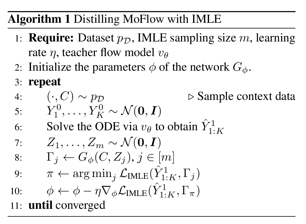
The IMLE distillation process is summarized in Algorithm 1. Lines 4–6 describe the standard ODE-based sampling of the teacher model, which produces $K$ correlated multi-modal trajectory predictions \(\hat{Y}^1_{1:K}\) conditioned on the context $C$. A conditional IMLE generator $G_\phi$ then uses a noise vector $Z$ and context $C$ to generate $K$-component trajectories $\Gamma$, matching the shape of \(\hat{Y}^1_{1:K}\).
Unlike direct distillation, the conditional IMLE objective generates more samples than those available in the teacher’s dataset for the same context $C$. Specifically, $m$ i.i.d. samples are drawn from $G_\phi$, and the one closest to the teacher prediction \(\hat{Y}^1_{1:K}\) is selected for loss computation. This nearest-neighbor matching ensures that the teacher model’s modes are faithfully captured.
To preserve trajectory multi-modality, we employ the Chamfer distance
where $\Gamma^{(i)} \in \mathbb{R}^{A \times 2T_f}$ is the $i$-th component of the IMLE-generated correlated trajectory.
Nonetheless, the acceleration of diffusion-based models—particularly through distillation—is evolving rapidly. Our work with IMLE is just one attempt in this direction, and we are actively exploring further improvements to extend its applicability to broader domains.
Summary
We reviewed the challenges and engineering insights gained from developing conditional generative models for motion prediction, primarily drawing on our previous works
From these experiences, we identified two useful engineering practices:
- Data-space predictive learning objectives outperform denoising-based approaches, leading to more stable convergence.
- Joint multi-modal learning losses that integrate regression and classification more effectively capture trajectory diversity.
In addition, we explored the IMLE distillation technique to accelerate inference by compressing iterative processes into a one-step generator, while preserving multi-modality through Chamfer distance losses.