On the Permutation Invariance of Graph Generative Models
This blog post discusses the permutation invariance principle of graph generative models, which has often been taken for granted in graph-related tasks. While permutation symmetry is an elegant property of graph data, there is still more to learn about its empirical implications.
Introduction
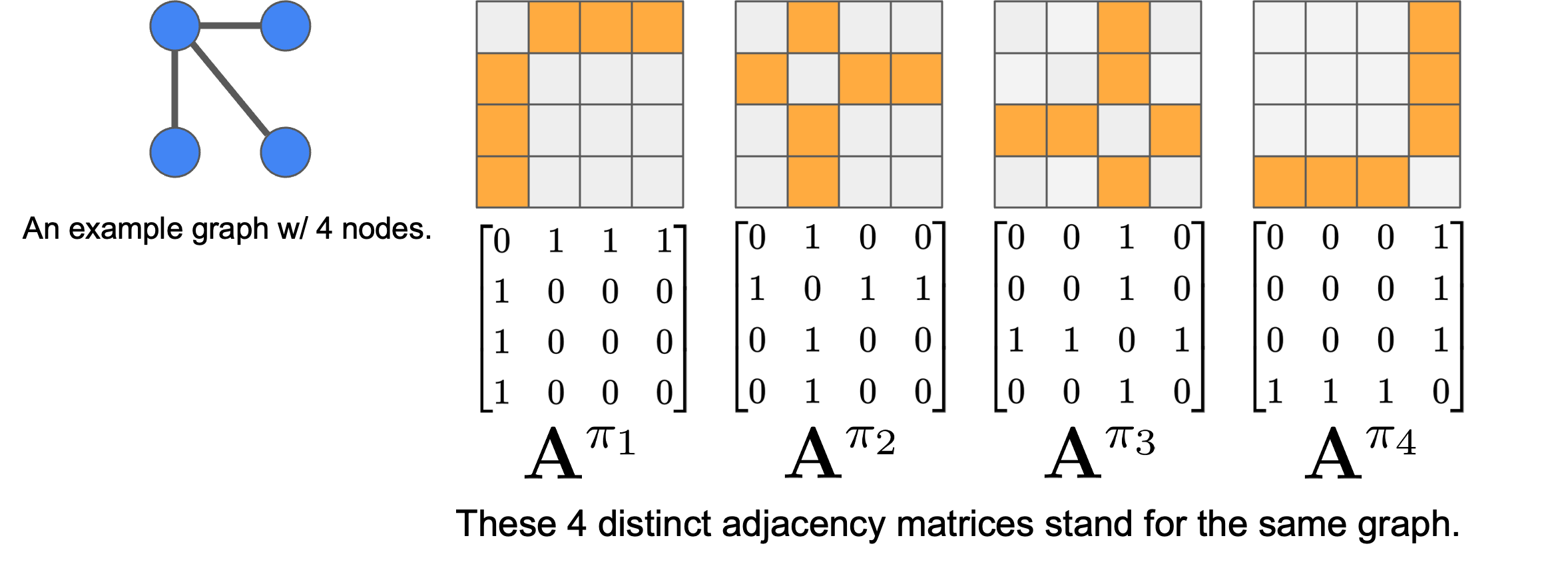
Graphs are ubiquitous mathematical objects that arise in various domains, such as social networks, protein structures, and chemical molecules. A graph can be formally represented as a set of nodes $V$, optionally associated with node features $X$, and a set of edges $E$. Its topology is commonly expressed using an adjacency matrix $A$.
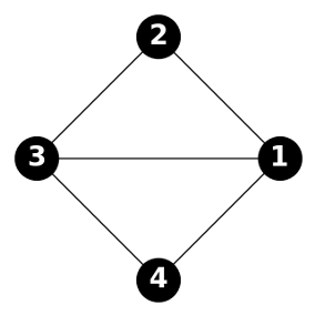
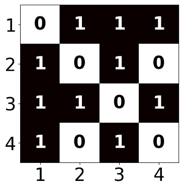
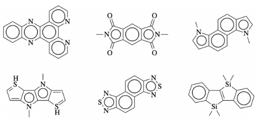
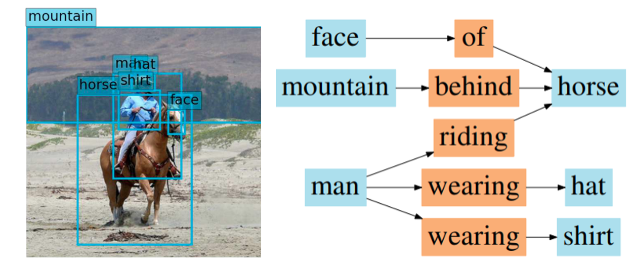
The goal of graph generative models is to generate novel graph samples that resemble those drawn from the true data distribution. Graphs can be stored in several ways in computational systems, including tree-based structures
Permutation Symmetry for Graph Representation Learning
Permutation symmetry (i.e., permutation invariance and equivariance) is a fundamental design principle in graph representation learning tasks. Below, we provide a quick recap of the key ideas using resources from
A straightforward idea for constructing a deep neural network on graphs is to use the adjacency matrix directly as input. For instance, to obtain an embedding of the entire graph, one could flatten the adjacency matrix and pass it through a multi-layer perceptron (MLP):
\[\mathbf{z}_G = \text{MLP}({A}[1] \oplus {A}[2] \oplus \dots \oplus {A}[ \vert V \vert]),\]where ${A}[i] \in \mathbb{R}^{\vert V \vert}$ corresponds to the $i$-th row of the adjacency matrix, and $\oplus$ denotes vector concatenation. The drawback of this method is that it relies on the arbitrary ordering of the nodes in the adjacency matrix. Consequently, such a model is not permutation invariant.
A fundamental requirement for graph representation learning models is that they should exhibit permutation invariance (or equivariance). Formally, a function $f$ that processes an adjacency matrix ${A}$ should ideally satisfy one of the following conditions:
\[\begin{aligned} f({PAP}^\top) &= f({A}) \quad \text{(Permutation Invariance)} \\ f({PAP}^\top) &= {P} f({A}) P^\top \quad \text{(Permutation Equivariance)} \end{aligned}\]where ${P} \in \mathbb{R}^{\vert V \vert \times \vert V \vert}$ represents a permutation matrix
- Permutation invariance implies that the function’s output does not change with different node orderings in the adjacency matrix.
- Permutation equivariance means that permuting the adjacency matrix results in a correspondingly permuted output of $f$.

Specifically, node- and edge-level tasks require permutation equivariance, while graph-level tasks require permutation invariance. A well-designed Graph Neural Network (GNN) should generalize across arbitrary permutations of node and edge indices. This ensures that outputs are symmetric with respect to node ordering in the input graph data. It has two key advantages: (i) during training, the model avoids the need to consider all possible node orderings (exhaustive data augmentation), thereby reducing learning complexity and enjoying theoretical benefits
Rethinking Invariance Principle for Generative Models
For graph generative models, permutation symmetry boils down to the invariance of the learned probability distribution. Namely, $p_\theta(\hat{A}) = p_\theta(P \hat{A} P^\top)$ must hold for any valid permutation matrix $P$. Two adjacency matrices related by such a permutation are said to be isomorphic
Invariance of Probability Distributions
Theorem 1 (from
). If $ \mathbf{s} : \mathbb{R}^{N \times N} \to \mathbb{R}^{N \times N} $ is a permutation equivariant function, then the scalar function $ f_s = \int_{\gamma[\mathbf{0}, {A}]} \langle \mathbf{s}({X}), \mathrm{d}{X} \rangle_F + C $ is permutation invariant, where $ \langle {A}, {B} \rangle_F = \mathrm{tr}({A}^\top {B}) $ is the Frobenius inner product, $ \gamma[\mathbf{0}, {A}] $ is any curve from $ \mathbf{0} = \{0\}_{N \times N} $ to $ {A} $, and $ C \in \mathbb{R} $ is a constant.
We refer readers to
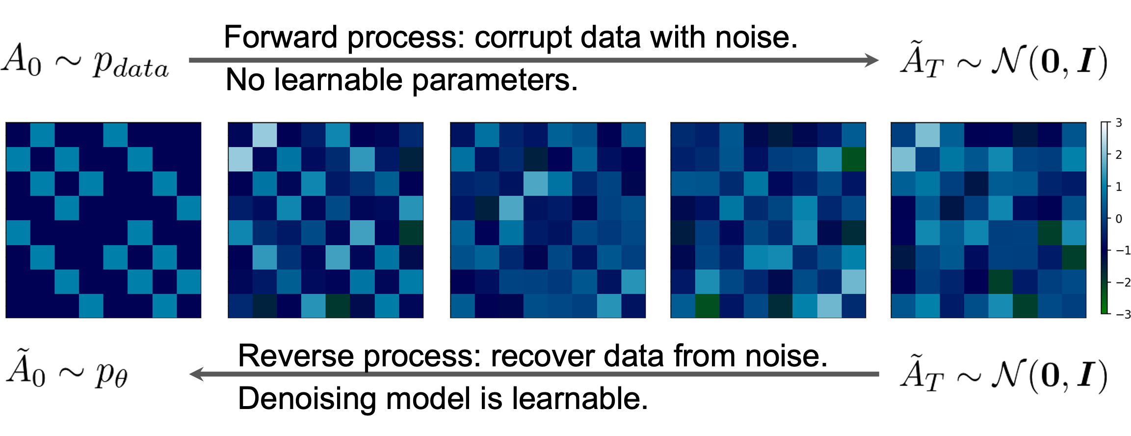
Thus, if the learned gradient of the log-likelihood $\mathbf{s}_\theta(A) = \nabla_{A} \log p_\theta(A)$ is permutation equivariant, then the implicitly defined log-likelihood function $\log p_\theta(A)$ is permutation invariant, according to Theorem 1, as given by the line integral of $\mathbf{s}_\theta(A)$:
\[\log p_\theta({A}) = \int_{\gamma[0, {A}]} \langle \mathbf{s}_\theta({X}), \mathrm{d} {X} \rangle_F + \log p_\theta(\mathbf{0}).\]Based on this theorem, as long as the score estimation neural network (equivalently, diffusion denoising network) is permutation equivariant, we can prove that the learned probability distribution is permutation invariant. Later works such as GDSS
Implications on Scalability
While it is appealing to design a provably permutation invariant graph generative model, we find the empirical implications of this property are not as straightforward as one might expect.
Theoretical Analysis
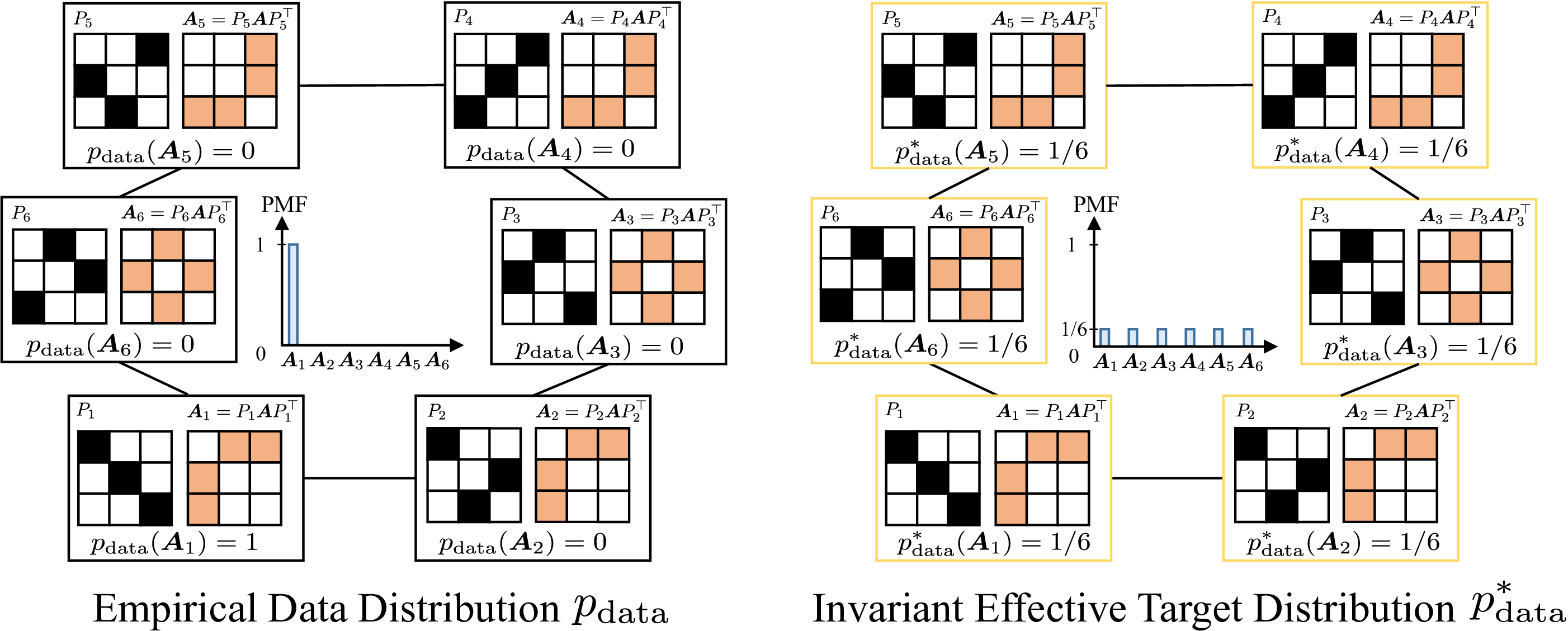
Here we provide a simple example to illustrate the potential challenges of learning permutation invariant graph generative models. As shown in the above figure, the empirical graph distribution $p_{\text{data}}$ (i.e., the observed training samples) may only assign a non-zero probability to a single observed adjacency matrix in its isomorphism class.
The ultimate goal of a graph generative model is to match this empirical distribution, which may be biased by the observed permutation. However, the target distribution that generative models are trained to match may differ from the empirical one, depending on the model design w.r.t. permutation symmetry.
For clarity, we define the effective target distribution as the closest distribution (e.g., measured in total variation distance) to the empirical data distribution achievable by the generative model, assuming sufficient data and model capacity.
Formally, given a training set of adjacency matrices $\{A_i\}_{i=1}^m$ with $N$ nodes , we define the union of their isomorphism classes as $\mathcal{A}^* = \bigcup_{i=1}^m \mathcal{I}_{A_i}$. Each isomorphism class $\mathcal{I}_{A_i}$ represents all adjacency matrices that are topologically equivalent to $A_i$ but may have different matrix representations. The corresponding effective target distribution distribution is
\[p_{\text{data}}^*(A) = \frac{1}{Z} \sum_{A^* \in \mathcal{A}^*} \delta(A - A^*),\]where $Z = \vert \mathcal{A}^* \vert = O(n!m)$ is the normalizing constant. Note that $Z = n!m$ may not always be achievable due to graph automorphisms
Lemma 2 (from
). Assume at least one training graph has $\Omega(n!)$ distinct adjacency matrices in its isomorphism class. Let $\mathcal{P}$ denote all discrete permutation-invariant distributions. The closest distributions in $\mathcal{P}$ to $p_{\text{data}}$, measured by total variation, have at least $\Omega(n!)$ modes. If, in addition, we restrict $\mathcal{P}$ to be the set of permutation-invariant distributions such that $p(A_i) = p(A_j) > 0$ for all matrices in the training set $\{A_l\}_{l=1}^m$, then the closest distribution is $\arg\min_{q \in \mathcal{P}} TV(q, p_{\text{data}}) = p_{\text{data}}^*.$
Under mild conditions, $p_{\text{data}}^*(A)$ with $O(n!m)$ modes, which is defined above, becomes the effective target distribution, which is the case for permutation invariant models using equivariant networks. In contrast, if we employ a non-equivariant network (i.e., the learned density is not invariant), the effective target distribution becomes $p_{\text{data}}(A)$, which only has $O(m)$ modes. While we discuss the number of modes from a general perspective, the analysis is also relevant to diffusion models
Empirical Investigation
In practice, we typically observe only one adjacency matrix from each isomorphism class in the training data $\{A_i\}_{i=1}^m$. By applying permutation $n!$ times, one can construct $p_{\text{data}}^*$ (invariant distribution) from $p_{\text{data}}$ (non-invariant distribution).
We define a trade-off distribution, called the $l$-permuted empirical distribution:
\[p_{\text{data}}^l(A) = \frac{1}{ml} \sum_{i=1}^{m} \sum_{j=1}^{l} \delta(A - P_j A_i P_j^{\top}),\]where $P_1, \ldots, P_l$ are $l$ distinct permutation matrices. The construction of $p_{\text{data}}^l$ has the following properties: (1) $p_{\text{data}}^l$ has $O(lm)$ modes governed by $l$; (2) With proper permutations, $p_{\text{data}}^l = p_{\text{data}}$ when $l=1$; (3) $p_{\text{data}}^l \approx p_{\text{data}}^*$ when $l=n!$ (identical if no non-trivial automorphisms). We use $p_{\text{data}}^l$ as the diffusion model’s target by tuning $l$ to study the impact of mode count on empirical performance.
The experimental setup is as follows. We use 10 random regular graphs with 16 nodes, with degrees in $[2, 11]$. The parameter $l$ ranges from 1 to 500, and all models are trained to convergence. For baselines, we consider invariant models for $p_{\text{data}}^*$: DiGress
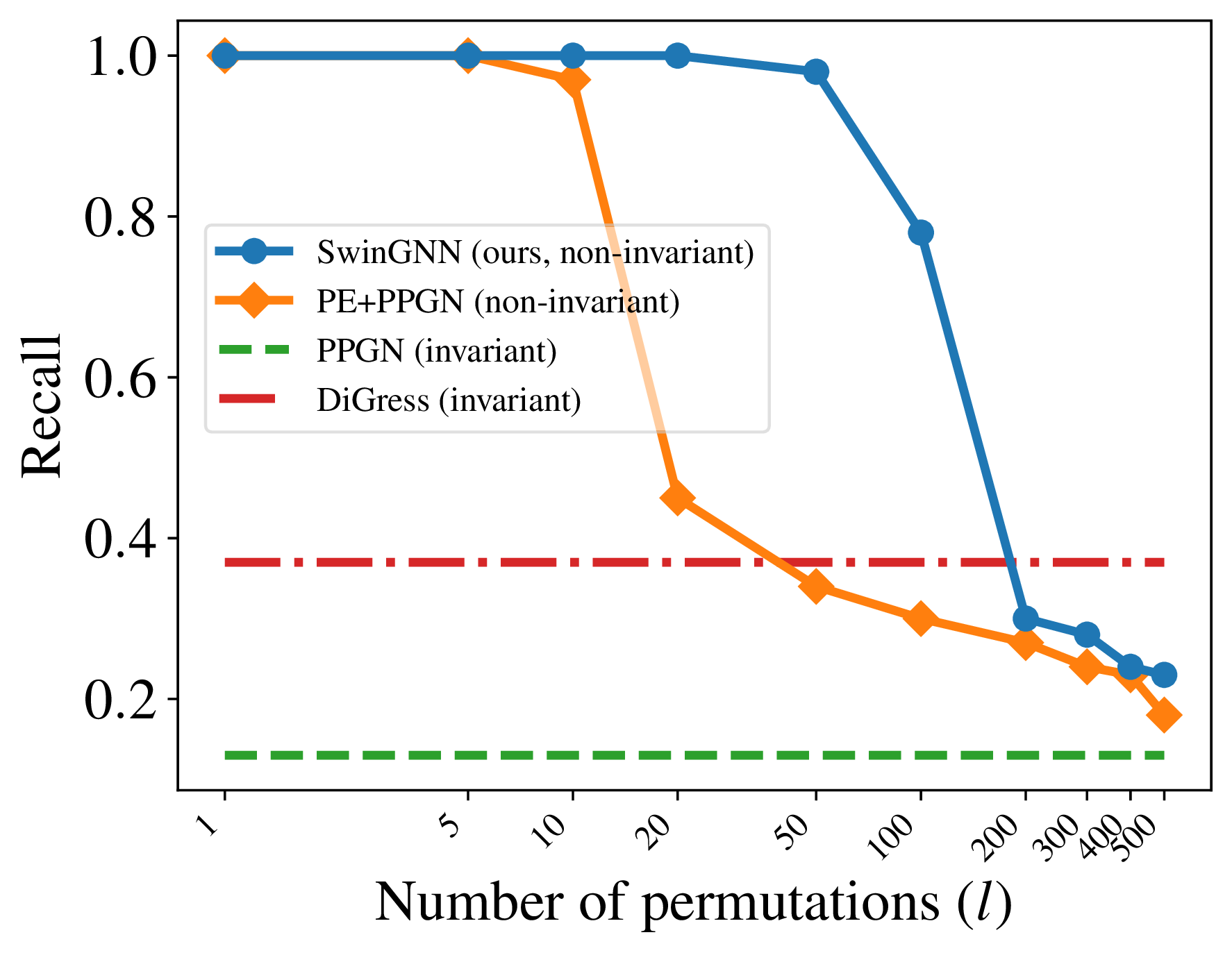
As shown in the plot above, invariant models such as DiGress and PPGN consistently fail to achieve high recall. In contrast, non-invariant models perform exceptionally well when $l$ is small, where only a few permutations are imposed, but their sample quality degrades significantly as $l$ increases, reflecting the difficulty of learning from distributions with many modes. Importantly, in practice, one typically sets $l=1$ for non-invariant models, which often leads to empirically stronger performance than their invariant counterparts.
Post-processing to Reclaim Sample Invariance
While non-invariant models often perform better empirically, they cannot guarantee permutation-invariant sampling. To bridge this gap, we propose a simple and provable trick: apply a random permutation to each generated sample, which yields invariant sampling at no extra cost.
Lemma 3 (from
). Let $A$ be a random adjacency matrix distributed according to any graph distribution on $n$ vertices. Let $P_r \sim \mathrm{Unif}(\mathcal{S}_n)$ be uniform over the set of permutation matrices. Then, the induced distribution of the random matrix $A_r = P_r A P_r^{\top}$, denoted as $q_\theta(A_r)$, is permutation invariant, i.e., $q_\theta(A_r) = q_\theta(P A_r P^{\top}), \forall P \in \mathcal{S}_n$.
This trick applies to all generative models. Importantly, the random permutation preserves the isomorphism class: $q_\theta$ is invariant but covers the same set of isomorphism classes as $p_\theta$. Thus, graphs from $q_\theta$ always have isomorphic counterparts under $p_\theta$.
In summary, there are two key observations: (1) invariant models ensure invariant sampling but may harm empirical performance, and (2) invariant sampling does not require invariant models.
Additional Experimental Results
Motivated by the aforementioned analysis, we design a new diffusion model that combines non-invariant objectives with invariant sampling to better capture graph distributions.
click here for more details on model design
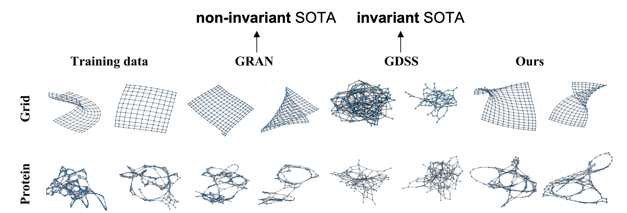
From the qualitative results, especially on the grid dataset, we can clearly see the difference between the non-invariant and invariant models, compared with then-SOTA models GRAN
We also show the models’ superiority on the quantitative results on more synthetic and real-world datasets. The metrics are computed by maximum mean discrepancy (MMD) metrics characterizing graph structure properties, such as degree distributions. Please refer to the expandable box below and the original paper

click here for more quantitative results

Discussion with Recent Works
It is interesting to see concurrent works adopting similar principles or arrive at similar findings regarding the permutation invariance property for generative models in the graph domain.
For instance, AlphaFold 3 (2024)
The diffusion module operates directly on raw atom coordinates, and on a coarse abstract token representation, without rotational frames or any equivariant processing.
AlphaFold 3 indeed applies data augmentation to encourage equivariance but does not impose this condition through network design.
Similarly, DiffAlign
More interestingly, research from the optimization perspective also addresses this problem and provides fresh insights, studying the relationship between intrinsic equivariance and data augmentation
Summary
This post examines the role of permutation invariance in graph generative models. While symmetry is essential in graph representation learning, enforcing it in generative models can make learning harder by introducing exponentially many modes. Empirical results show that non-invariant models often outperform invariant ones, especially with limited permutations. A simple post-processing trick—random permutation—restores invariant sampling without requiring invariant model design. Building on this, we propose non-invariant graph generative models that achieve strong performance on synthetic and real-world datasets